I started working with high level languages when I realized I was spending far too much time writing Fortran and C language programs as a part of engineering analyses, test data reduction, and continuing education. I searched for a better engineering programming tool; except for Matlab, and some Matlab-like programs (all commercial), I came up empty-handed (this was in 1989). I did not feel Matlab’s language design was powerful enough, but I would have used it had it been lower in cost and available on more platforms. I diverted my “off-hour” studies to interpreter construction, and started prototyping Rlab. Within a year, I released version 0.10 to the Internet for comment. Now, almost five years later, Rlab has undergone significant changes and improvements primarily due to excellent assistance from users around the world.

Rlab does not try to be a Matlab clone. Instead, it borrows what I believe are the best features of the Matlab language and provides improved language syntax and semantics. The syntax has been improved to allow users more expression and reduce ambiguities. The variable scoping rules have been improved to facilitate creation of larger programs and program libraries. A heterogeneous associative array has been added to allow users to create and operate on arbitrary data structures.

The term “high level language” has many different connotations. In the context of Rlab it means that variables are not explicitly typed or dimensioned. A variable’s type and dimension are inferred from usage, and can be arbitrarily changed during a program’s execution. This automatic typing and dynamic allocation free the scientific programmer from many of the more time consuming programming duties normally associated with languages like C or Fortran.

In Rlab’s case, high level also means interactive. Since one of the purposes is to provide convenient means for data manipulation and visualization, the program can be run in either batch or interactive mode. Typing rlab at the shell prompt starts the program. Rlab gives the user the command line prompt prompt >, from whence program statements are issued and executed.

What do you get? What does it cost? Most people find that they can develop a working program far faster than with C or Fortran. Furthermore, the built-in graphics capabilities and interactive mode of operation promote experimentation and exploration of data and methods. The price you pay is slower program execution in some instances. Performance tests between compiled and interpreted languages usually show the compiled language to be faster in all respects. If your Rlab program uses scalar operations exclusively, and uses none of the built-in linear algebra functions, then it will be substantially slower than the Fortran or C version. However, if you take advantage of Rlab’s optimized array operations, built-in linear algebra and utility functions, you may find that Rlab will perform quite well.

Although I cannot provide a complete introduction in a single article, I can show you enough of the language to help you decide if it is something that you would want to try. A more complete introduction is provided in “The Rlab Primer”, which is included in the source and binary distributions.

The numeric array, or matrix, is the most commonly used data type. The numeric array can be one-dimensional (a vector) or two-dimensional. Most often, matrices are created by reading data from another program or from a file. For simpler examples, we will create our matrices interactively. Array/matrix syntax uses square brackets, [ ], like the C language, to delimit the matrix, and semi-colons to separate each row from the next. So, to create a matrix within Rlab, the user types:

> a = [1, 2; 3, 4]

Which provides the following response:

  a =
        1          2
        3          4

Matrix referencing and assignment uses the following syntax:

> a[1;] = 2 * a[2;2,1]
 a =
        8          6
        3          4

The semi-colon delimits row and column specifications. The absence of a row or column specification selects all of the rows or columns. Additionally, the user can specify particular indices, or combinations of indices, in any order. In the previous example, a[2;2,1] selects the second row of a, and the second and first columns (in that order) of that row. Therefore, a[2;2,1] evaluates to [4,3]. This quantity is then multiplied by 2, and the result is assigned to the first row of a.

In this article real numbers will be used in all of the examples. However, Rlab can deal with complex numbers equally well. To enter a complex number, the imaginary constant i or j is used (don’t worry, you can still use i and j as variables). For example: a = 1 + 2j creates the complex number with real part 1 and imaginary part 2. All numeric operators and functions (where they make sense) work with complex values as well as real values.

The traditional numeric operators are overloaded. When working with scalar operands, the results are what most people would expect. However, when working with array/matrix operands, the numeric operators behave differently. Addition and subtraction function in an element-by-element sense between the two operands. The multiplication operator * performs the matrix inner-product. To illustrate:

> a = [ 1 , 2 , 3 ];
> b = [ 4 , 5 , 6 ];
> a + b
        5          7          9
> a' * b
        4          5          6
        8         10         12
       12         15         18
> a * b'
       32

Note (in the first two lines) that a ; at the end of a statement suppresses printing the result. The division operator / performs traditional division on scalar operands, and solves sets of simultaneous linear equations with matrix/vector operands. A set of element-wise operators exist to perform element-by-element operations between arrays. The element-wise operators are two-symbol operators; the first symbol is always a . so the element-wise division operator is ./ and the element-wise multiplication operator is .*:

> a = [1,2,3;4,5,6];
> b = 1./a
 b =
        1        0.5      0.333
     0.25        0.2      0.167
> a.*b
        1          1          1
        1          1          1

In addition to the numeric class of data, there is a string class. String arrays/matrices are handled in exactly the same way as numeric arrays:

> s = ["how", "to create" ;
>      "a string", "within rlab"]
 s =
how          to create
a string     within rlab

As you can see, string arrays consist of arbitrary length strings. There are no restrictions upon the relative size of strings in an array. Strings can be concatenated with the + operator. The other (traditionally numeric) operators do not operate on string arrays.

One of the benefits of the C language is the ability to create data structures to suit a particular programming task. Rlab offers a similar programming construct called a list. In their simplest form, lists are single-dimension associative arrays. However, since list elements can be strings, numbers, arrays, functions, and other lists, they provide a powerful multi-dimensional tool. Lists are created in a manner similar to numeric arrays:

> l = << 3*pi ; rand(3,4) ;
>        type = "my-list" >>
 l =
   1            2            type

The << >> delimiters contain the list elements, with ; separating the elements. The = is used to assign an index name (which cannot be numeric) to an element, as in the third element of the list above. If a list element is not assigned an index, then a numeric value is assigned by default, as in the first two elements.

Elements of a list are referenced by their index: l.[“type”] returns the string “my-list”, and l.[1] returns the value of 3*pi. In the case of explicit index names, shorthand notation can be used: l.type will also return the string “my-list”.

List indices can be replaced by expressions that evaluate to a string, or a numeric-scalar, allowing users access to selected elements in an automated fashion. If index is a variable containing the string “type”, the expression l.[index] will access the type element and return the string “my-list”. If index contains the number 1, l.[index] will return 9.42. Lists will be discussed again later in the article.

Rlab provides the user with conditional and if-statements for conditional execution, for and while-statements for looping capability, and functions or subroutines. These capabilities will be introduced as we proceed with some examples.

Rlab functions are a little unusual, and deserve some attention. Functions, while not first class, are objects, referred to with variables. Thus, to create and save a function, it must be assigned to a variable. The function argument passing and variable scoping rules were designed to facilitate creation of larger programs and program libraries. Our first example, integrating an ordinary differential equation will illustrate some of these features.

A popular example is Van der Pol’s equation, because it is simple, non-linear, and it demonstrates limit-cycle oscillation. Rlab has a built-in integration engine, and several “rfile” integrators. An rfile is a file that contains an Rlab program or statements. The integration function needs as input: a function that returns the value of the derivative, values defining the start and end of the integration interval, and the initial conditions.

The entire problem could be performed interactively. However, I have chosen to put the program in a file (int.r). This allows me to edit and re-execute without a lot of repetitive typing. For this article, I have used the shell-escape feature (\ in the first column) to cat the file through pr to generate Listing 1.

Listing 1. ODE Listing

> \cat int.r | pr -t -n:2 -
 1:vdpol = function ( t , x )
 2:{
 3:  global (mu)
 4:  xd[1] = x[1] * mu*(1-x[2]^2) - x[2];
 5:  xd[2] = x[1];
 6:  return xd;
 7:};
 8:
 9:mu = 0.1;
10:t0 = 0; tf = 30; dt = 0.011;
11:x0 = [-5; 5];
12:
13:tic();
14:out = ode( vdpol, t0, tf, x0, dt );
15:printf("ODE time: %10.3f\n", toc());

Since the ode function integrates first order differential equations, we must write Van der Pol’s equation:

as two first order equations:

The function, which calculates and returns,

is written and assigned to the variable vdpol. After the function is defined, variables t0, the integration start time; tf, the integration final time; and x0, the initial conditions, are initialized (lines 9-11). tic and toc, builtin timing functions, are used around the call to ode to tell us how long the integration takes.

Once this file is finished, the following command will execute it, as if each line was entered from the prompt.

"> rfile int
ODE time:      0.620

This simple problem runs fairly fast. The output from ode, a matrix of the time-dependent values of,

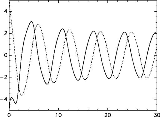
is stored in the variable out (line 14). Convenient data visualization is a real plus when investigating the behavior of differential equations. In this instance we would like to look at

(x) and

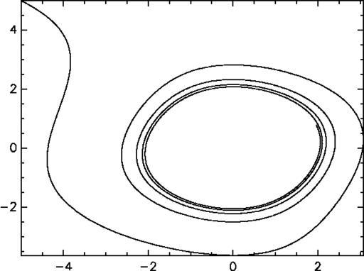
(xd) versus time. We would also like to look at the phase-plane for this problem, which is a plot of

versus.

We can do this with the plot function, which plots matrix columns. If the input to plot is a single-column matrix, the matrix row indices are plotted against the abscissa-axis, and the matrix column elements are plotted against the ordinate-axis. If the input to plot is a N-column matrix, then the values in the first column are plotted against the abscissa-axis, and the remaining columns are each plotted against the abscissa-axis.

Figure 1. Integration Example, Time-Series

A plot, similar to Figure 1, can be created with the command plot(out);. Since the first column of out is time, and the second and third columns are x and xd, all we have to do is give the unaltered matrix to plot. If we want to plot the phase-plane, as in Figure 2, we need to specify that we want the third column plotted against the second. To do this simply extract the second and third columns from out like so: plot(out[;2,3]);

The Plplot graphics library provides the builtin 2 and 3D graphics capability for Rlab. Builtin functions for most common graphics capabilities such as: 2D, 3D, mesh-plots, contour-plots, and histograms are supplied. Plplot supports most common graphics output devices, most notably X-Windows and PostScript.

It is possible that Plplot graphics may not be sufficient. In these cases the ability to get properly formatted data to another program is paramount. There are several methods of interfacing Rlab with other programs. Like most good Unix applications, Rlab will read from stdin and write to stdout. There are functions for writing matrices in ASCII format, as well as a C-like [f]printf function. There is also a system function that allows Rlab programs to do anything that can be done with the Unix shell. However, what makes interfacing with other programs easiest is the facility for writing to, and reading from a process (pipes).

The user-end of the I/O system was designed to be as simplistic as possible, without restricting capability for those who need it. Files and processes are identified with strings. Each function capable of reading or writing will open and close files as necessary. However, open and close functions are provided for special circumstances. There are several variations of read and write functions that understand all of Rlab’s internal data structures, and offer some degree of Matlab file compatibility. The getline and strsplt functions used for special ASCII input needs, a fread used for binary input, and a fprintf used for specially formatted output round out the I/O functions.

As you might expect, the strings “stdin”, “stdout”, and “stderr” point to their Unix system counterparts. Any function that performs file I/O can also perform process I/O through pipes, by simply replacing the filename string with a process-name string. A process-name string is a string that has a | as its first character. The rest of the string is any shell command. Rlab will create a pipe, forking and invoking the shell. The direction of the pipe is inferred from usage. This facility makes getting data to and from other programs rather simple. A good example is the Rlab-Gnuplot interface, which is written entirely in the Rlab language, using the process I/O capability to get data and commands to Gnuplot.

As a demonstration, we will explore process-I/O with a simple interface to the X-Geomview program. X-Geomview is a powerful 3-dimensional graphics engine, with an interactive GUI. X-Geomview can read data from files, and it can also read data/commands from stdin. X-Geomview uses Motif, but statically linked Linux binaries are available (in addition to the sources) from www.geom.umn.edu/software/geomview/docs/geomview.html.

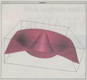
In this example I will generate the data for, and plot, the classic sombrero. The code is listed in Listing 2.

Listing 2. Geomview Example Listing

\cat geom-ex.r | pr -t -n:2 -
 1:N = 40;
 2:x = linspace(-1,1,N);
 3:y = x;
 4:z = zeros(N, N);
 5:
 6:for (i in 1:N)
 7:{
 8:  for (j in 1:N)
 9:  {
10:    r = sqrt(x[i]^2 + y[j]^2);
11:    z[i;j]=.4*(exp(-r*r)*cos(2*pi*r));
12:  }
13:}
14:
15:GM = "|/usr/local/bin/geomview -c -";
16:fprintf(GM,...
17: "(geometry rmesh { : rmesh })\n");
18:fprintf(GM,...
19: "(read geometry { define rmesh\n");
20:fprintf(GM,"MESH\n");
21:fprintf(GM,"%i %i\n", N, N);
22:
23:for (i in 1:x.n)
24:{
25:  for (j in 1:y.n)
26:  {
27:    fprintf(GM,"%f %f %f\n",...
28:            x[i],y[j],z[i;j]);
29:  }
30:}
31:
32:fprintf(GM, "})\n");

The data for the example is completed by line 14; from there on, we are simply sending the data to the X-Geomview process. The variable GM holds a string, whose first character is a |, indicating a process to the remainder of the string should be opened. The following statements (lines 16-21) send object definition to X-Geomview, and lines 23-30 include the nested for-loops that send the polygon vertex coordinates to X-Geomview. A snapshot of the X-Geomview window containing the result is presented in Figure 3. Of course, a much better way to make this type of plot is to create a function that automates the X-Geomview interface (this will be included in the next release of Rlab).

Figure 3. Geomview Example

High level languages are great for prototyping a procedure, but often fall just short of useful when it comes time to use the program in a “production” situation. In this example we will pretend that we have just developed a method for computing time-frequency distributions. Actually we are going to use Rene van der Heiden’s tfd function, which is derived from the information in Choi and Williams’ paper, “Improved Time Frequency Representation of Multicomponent Signals Using Exponential Kernels”.

Now we want to use tfd to process a large amount of data. Since tfd executes reasonably fast, we would hate to have to re-code it in some other language just to be able to handle a large amount of data. Suppose you have many files of time-history data that you wish to “push” through tfd. Some of the files contain a single matrix of event data, while others contain several matrices of data. You would like to be able to write a program that could process all such files with a minimum of user intervention. The difficulty for some languages is the inability to manipulate variable names, and isolate data.

Rlab addresses this problem with lists. Lists allow the creation, and isolation of arbitrary data structures, and provide a mechanism for systematically manipulating workspace variables, and variable names. I showed earlier how list elements could be accessed with strings. Lists can also be indexed with a string variable, or for that matter, any expression that evaluates to a string.

The interesting thing I have not disclosed yet is that the entire workspace can be treated as a list! Access to the workspace is granted through the special symbol $$. You can use $$ as the name of a list-variable. For example, you could use the cosine function like: $$.[“cos”](pi), or: $$.cos(pi). The first method offers the most flexibility. Now that we know about this special feature, we can handle our problem with relative ease. The program will read each file that contains data (they match the pattern *.dat) one at a time, compute the time-frequency distribution, and save the distribution for each set of data in the workspace. When processing is complete, the new workspace will be saved in a single file for later use.

Listing 3. TFD Listing

> \cat list-ex.r | pr -t -n:2
 1:require tfd
 2:
 3:i = 1;
 4:files = "|ls *.dat";
 5:
 6:#
 7:# Read the data from each file...
 8:#
 9:
10:while(length(line = getline(files)))
11:{
12:  filenm[i] = line.[1];
13:  readb(filenm[i], $$.[filenm[i]]);
14:  i++;
15:}
16:
17:close (files);
18:
19:#
20:# Now work on each list, computing
21:# the TFD for each matrix in each list...
22:#
23:
24:for (i in filenm)
25:{
26:  for (j in members ($$.[i]))
27:  {
28:    $$.[i].[j+"y"] = tfd ($$.[i].[j]);
29:  }
30:}
31:
32: save("tfd.dat")

The program just described is contained in Listing 3. There are several things I should point out:

There are many features, functions, and user-contributed programs that I have not discussed. Of special note are the extensive set of linear algebra functions. Rlab provides a very convenient interface to the LAPACK, FFTPACK, and RANLIB libraries available from Netlib and Statlib.

By now you have should have seen enough of the language to decide whether it is worth the effort to try it out. If you would like to find out more about it you can check out: www.eskimo.com/~ians/rlab.html. The Linux binaries of Rlab are now being distributed in RPM format, and are available at ftp://ftp.eskimo.com/u/i/ians/rlab/linux. Now that ELF distributions are available, and out of beta testing, and considering how much better dynamic linking is with ELF, Rlab binaries are built using the ELF object file format.

The Plplot graphics library is provided by Dr. Maurice LeBrun at the University of Texas. The underlying linear algebra subroutines (LAPACK, and the BLAS) are from the Netlib repository. And, of course, none of this would have been possible without GNU tools. There have been many other contributions to Rlab by various individuals over the years. The ACKNOWLEDGMENT file in the source distribution tries to mention everybody.

Rlab is available with over a hundred rfiles of various sorts, many contributed by users. Professor J. Layton, at Clarkson University, Potsdam NY, is in the process of finishing up the Rlab Controls Toolbox. A port of Professor Higham’s (University of Manchester/UMIST) Test Matrix Toolbox is also available. For more information go to www.eskimo.com/~ians/rlab.html